Tropical Events:
the solstices and equinoxes
This presentation is a simple layman’s study of some interesting aspects of Earth’s orbital history, especially concerning solstices and equinoxes, and the changing lengths of the days, seasons, and years. The charts below are from an Excel spreadsheet, created with an open source Excel Add-In, both of which I am making available at the end of this webpage: as I would have loved to have started out with something similar 10 years ago, when I first became interested in “the motions of the heavens” and the workings of the solar system.
My first inquiry concerned the “mean tropical year”: why does it change?
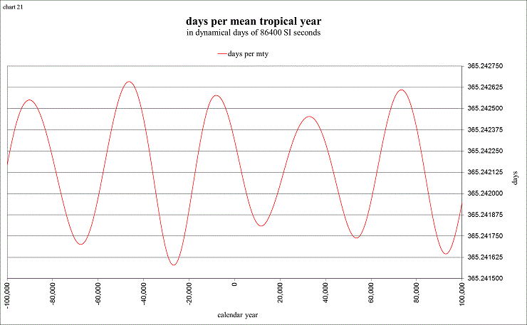
view larger→ mty.png
It is mostly due to the changing speed of the precession!
The rate of precession is shown below in arcseconds per Julian year (365.25 days), a standard time increment used by astronomers.
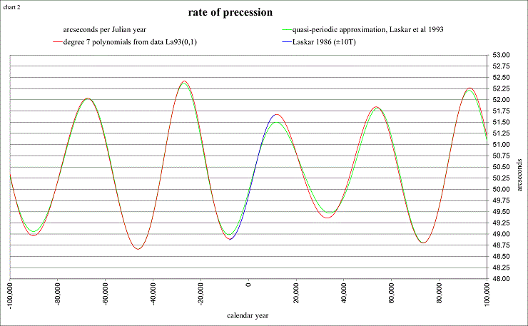
view larger→ precess.png
Comparison with the next chart shows us the relationship of the precession rate to the obliquity of the ecliptic (the tilt of our spin axis in relation to our orbital plane):

view larger→ obliq.png
The precession and the obliquity are from Jacques Laskar (et al 1993), an awesome astronomer at the Bureau des Longitudes in France who applies the concepts of Newton’s equations of motion to the entire solar system for millions and millions of years! He then approximates his results with one single equation (called a quasi-periodic approximation) that is very close to the “true solution”, at least for a few millions of years. This one for the precession and obliquity gives good results for 18 million years in the past, according to his solution usually designated La93(0,1), and it also gives good approximate results for 2 million years into the future. The Add-In can calculate with either the quasi-periodic approximation formulae, or from 7th-order polynomial expressions that interpolate the data from his La93(0,1) solution. The spreadsheet used to create these charts also uses the formulae from Laskar 1986 (valid for ±10,000 years from J2000), providing a comparison during the time period “closer to home”.
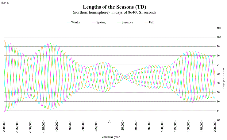
My next question concerned the lengths of the seasons: “why are they changing?”
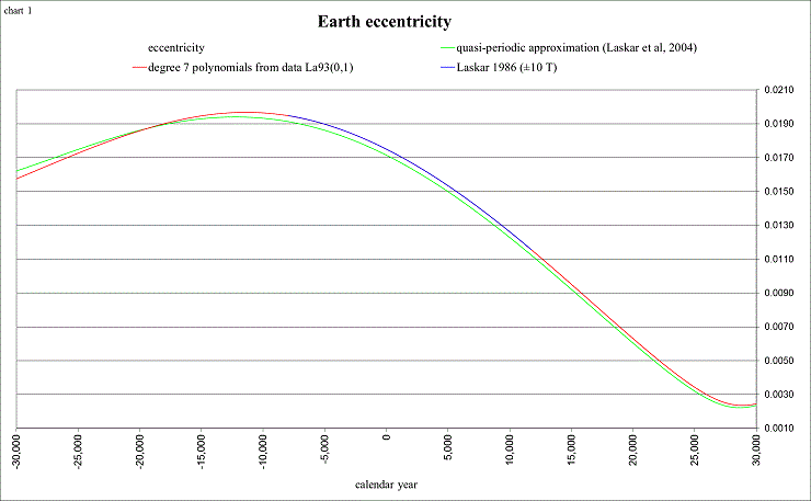
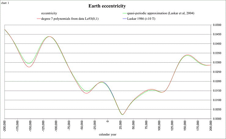
view larger→ ecc1.png
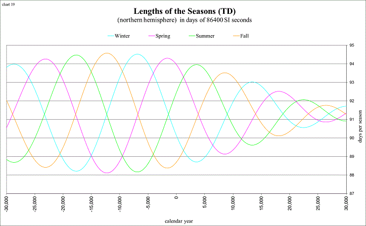
view larger→ seasons1.png
It is mostly due to the changing eccentricity and motion of the perihelion!
As the eccentricity approaches zero (circular orbit), the seasons become nearly equal.You can detect the motion of the perihelion from the previous chart, as it moves from season to season, causing that season to be “shortest”. The next chart shows the speed of the perihelion’s motion as the length of the anomalistic year:

view larger→ anom_yr.png
Laskar (et al 2004) has developed another approximation formula for both the eccentricity and perihelion, valid from −15M (million years ago) to +5M (million years in the future). Again the Add-In has retained good accuracy by interpolating Laskar’s 1993 data with polynomial expressions. The method used is on p.32 in the book “Astronomical Algorithms” by Jean Meeus (1998), referred to as “Lagrange’s interpolation formula”.
The relationship between the eccentricity and the lengths of the seasons is very interesting to study:
view larger→ ecc2.png
view larger→ seasons2.png
The method and formulae used for charting these lengths of the seasons is documented on page 6 of TEequation.pdf
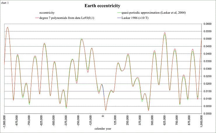
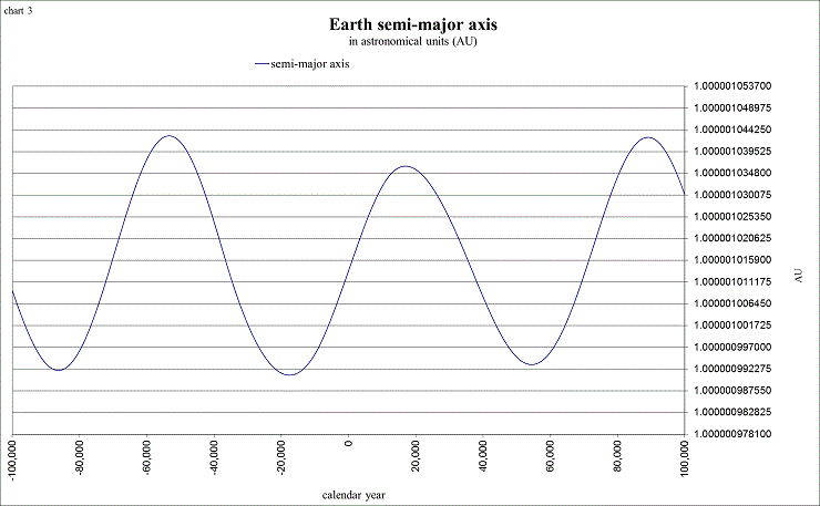
According to Laskar (2004), the eccentricity can reach as high as 0.063. This shows the variations for ±1 million years:
view larger→ ecc3.png
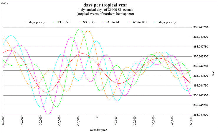
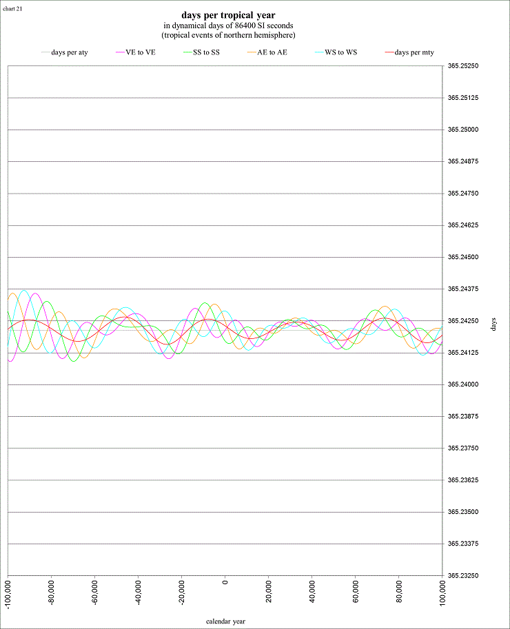
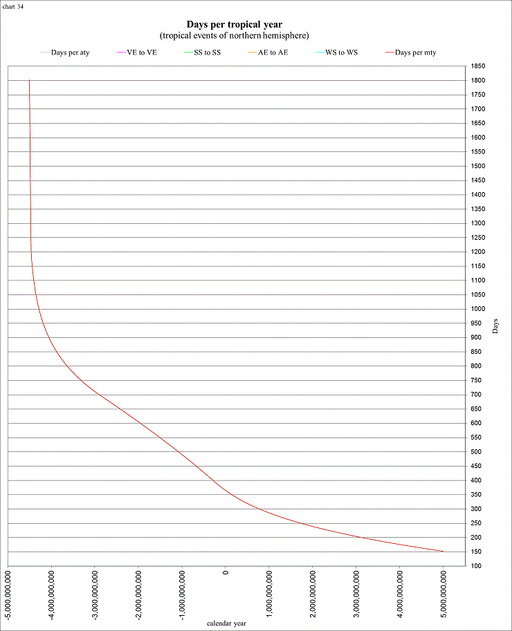
One of the most interesting things that I’ve learned is that not only is there the “mean tropical year”, there are 4 separate “true” tropical years, measured from vernal equinox to vernal equinox (VE to VE on the chart below), summer solstice to summer solstice (SS to SS), autumnal equinox to autumnal equinox (AE to AE), and winter solstice to winter solstice (WS to WS). The “names” of the seasons (and the tropical events) on these charts are those of the northern hemisphere (southern hemisphere readers should of course swap the names “winter” and “summer”, and also the names representing “spring” and “fall”).
view larger→ days_yr1.png
You can see from this chart how the “true” tropical years vary about the mean tropical year (mty), and how the mean tropical year varies about the “average” tropical year (aty). The average tropical year is determined from the “average” length of the sidereal year (~365.256362) and the “average” rate of precession (50.4712 arcseconds per Julian year, by use of the solution La93(0,1)), so that, for this study, the average length of the tropical year is ~365.242138.
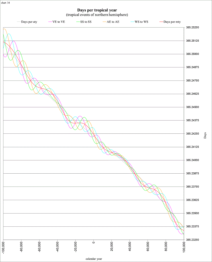
These previous charts are all in dynamical time, based on the well defined scientific second determined by atomic clocks, and counted in days of dynamical time equal to 86400 seconds per day. Let’s look at the lengths of the years during a longer time span and compare dynamical time to Universal time, which measures mean solar days of Earth rotations, known to be lengthening as Earth’s spin rate slows down, mostly due to tidal friction. To avoid confusion between the dynamical time scale of days and the Universal time scale of days, these charts have used days (with a lower case d) to designate dynamical time (TD), and Days (with a capital D) are used to designate mean solar days of Universal time (UT).
|
view larger→ days_yr2.png
|
view larger→ Days_yr3.png
|
What a difference! In this chart the dynamical time is converted to Universal time by showing the length of day (LOD) to be currently increasing by 1.7 ms/cy (milliseconds per century), a value determined by F. R. Stephenson (1997) from studies of eclipse records during the past 2700 years. This particular “scenario” in the spreadsheet shows the rate of change of LOD to be slowly increasing to a more scientifically expected rate of 2.3 ms/cy at ±100,000 yrs.
I also like to study the calendar, and the dates and times of solstices and equinoxes. These next charts show the dates and times of the vernal equinox every 10 years from −500 (501 BC) to +2000 (2000 AD) in both the Julian calendar and the Gregorian calendar, in the time zone of Rome (+1 hrs from Greenwich).
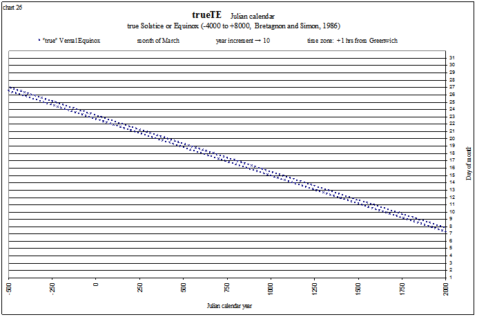
view larger→ trueVE_Julian.png
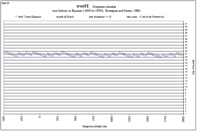
view larger→ trueVE_Gregorian.png
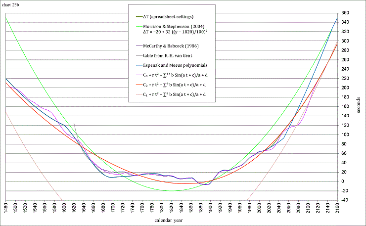
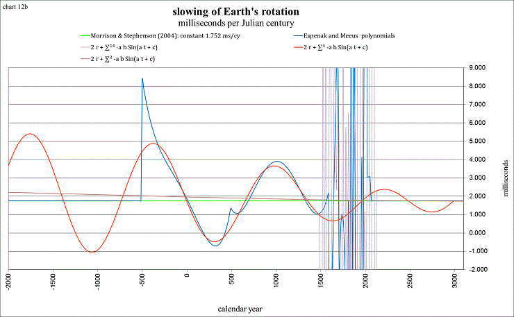
It is easy to see why we changed from the Julian to the Gregorian calendar! The dynamical times have been calculated by the method in the wonderfully compact book “Planetary Programs and Tables” by Pierre Bretagnon and Jean-Louis Simon (1986). They are supposed to be accurate to 0.0009 degree (within about 1⅓ minutes of time) from −4000 to +8000 AD. These times include the nutation in longitude (caused mainly by the Moon), and the aberration of light, so that they are the “observed” times of the tropical events. The calendar dates are calculated by algorithm from Meeus (1998). The value of ΔT (TD − UT) can be either from Morrison and Stephenson (2004), Espenak and Meeus (from NASA), a sum of sines, or any custom combination. The spreadsheet is currently set to use the Espenak and Meeus polynomials from −404 to +2003.5. C₂+ r t² + ∑⁴Sin(a t + c)/a + d is used from −6106 to −404 and from 2050 to 2668. To transition to this sum of 4 sines, from 2003.5 to 2050 a polynomial is used that also follows the data from the International Earth Rotation and Reference Systems Service (IERS) from 2000 to 2010:
63.9+0.164954*t-0.00281933*t^2+0.000879724*t^3-0.0000104809*t^4 where t = (JD -2451544.5)/365.2425
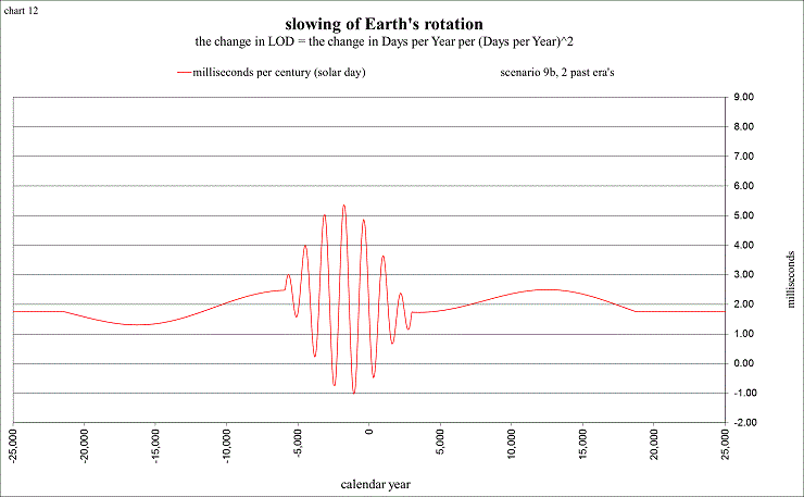
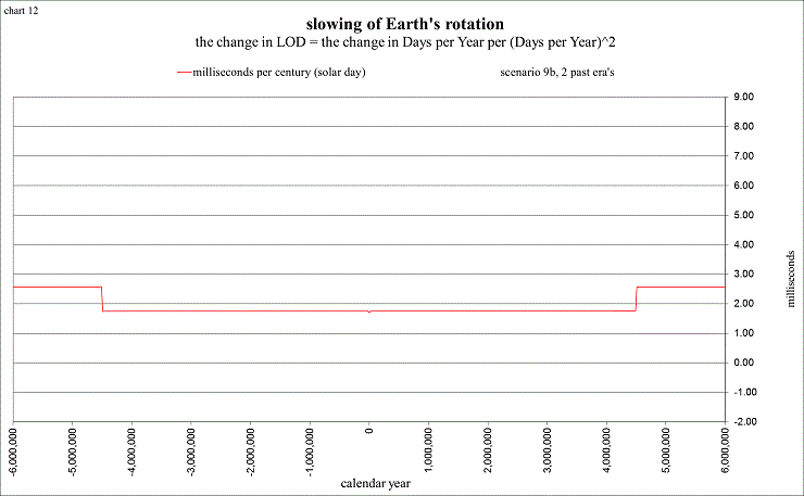
C₁+ r t² + ∑²Sin(a t + c)/a + d is used from −21,410 to −6106 and from 2668 to 18,749. Morrison and Stephenson (2004) is used from −4.5M to +4.5M, and the integral of an equation given by Deubner (1990) is used from −4.5G until +5G.
The sum of 14 sines is still under development, but a preliminary result is charted below, and the formula is documented on page 8 of TEequation.pdf
view larger→ deltaT.png
I also enjoy studying this rate of slowing for the entire history of the Earth-Moon system, from −4.5G (billions of years ago) until +5G (billion years in the future), when the Sun is expected to become a Red Giant, boiling the oceans and scorching the Earth! Intricately tied to the slowing of Earth’s spin rate is the Moon, due to the tidal friction that it causes. From our laws of physics (conservation of angular momentum), as the Earth’s spin angular momentum decreases, the Moon’s orbital angular momentum must increase, so that the total angular momentum is conserved. In order for the Moon’s orbital angular momentum to increase, the Moon must increase its distance from Earth, and that is why we measure the Moon to be moving away from the Earth at a rate of 3.82 ±0.07 centimeters per year (Dickey et al, 1994).
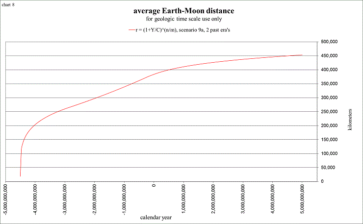
view larger→ E-M_km.png
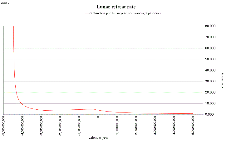
view larger→ Lunar_retreat.png
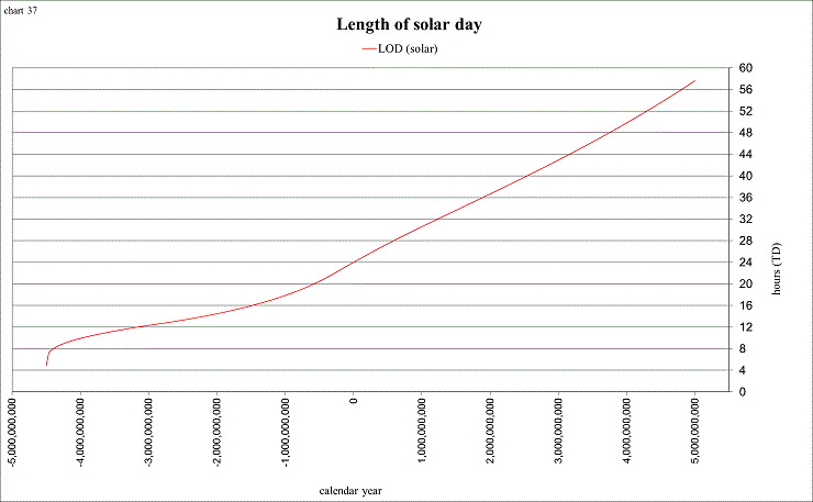
view larger→ LOD1.png
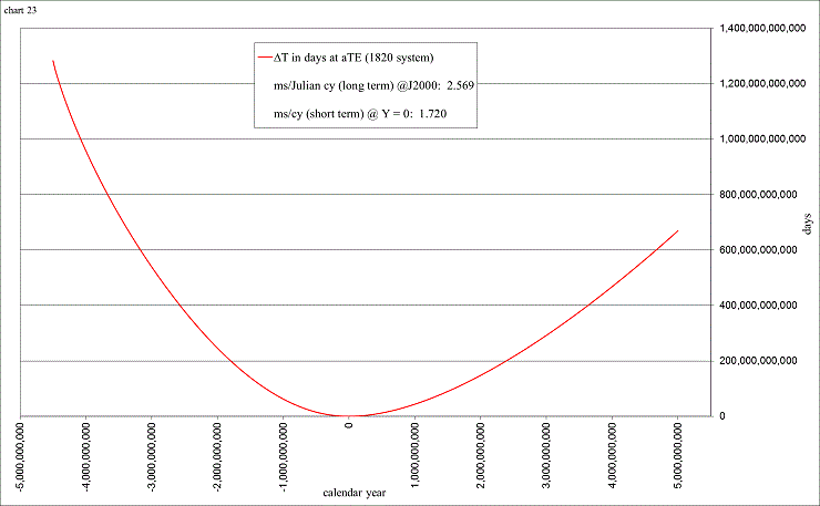
view larger→ deltaT2.png
view larger→ Days_yr4.png
These are of course speculative, as the true history of Earth-Moon distance and length of day (LOD) remains unknown. This is the reason for the different “scenarios” in the spreadsheet. They are easily changeable, so that you might find one to better suit your own ideas (as I am constantly changing my own!). Many of the parameters are also changeable, so that you can create your own custom scenario to depict a realistic Earth-Moon history. Some of the “targets” I like to consider are:
|
year |
Earth-Moon distance in kilometers |
Days per year |
source |
|
|
|
|
|
|
−4500M |
19,000 to 38,000 |
1800 to 1600 |
Canup (2004) |
|
−2450M |
330,000 |
512 |
Walker and Zahnle (1986) |
|
−2450M |
337,000 to 360,000 |
465 ±15 |
G.E. Williams (1989) |
|
−900M |
344,000 to 346,000 |
481 ±4 |
Sonett et al (1996) |
|
−900M |
364,700 |
419 |
G.E. Williams (2000) |
|
−620M |
369,100 to 372,900 |
400 ±7 |
G.E. Williams (2000) |
|
−250M |
372,600 |
397 |
Laskar et al (2004) |
|
+250M |
392,400 |
339 |
Laskar et al (2004) |
|
+5000M |
453,600? |
153.4 ±1.8 |
Néron de Surgy and Laskar (1997) |
Most of the scenarios use an equation for Earth-Moon distance given by Walker and Zahnle (1986), in which you can change the parameters. Then the Earth-Moon distance is applied to an equation given by Deubner (1990) to obtain Days per year. It is supposed to obey the conservation of angular momentum and include the effects of the solar tides. Some parameters of this equation are also changeable. The integral of Deubner’s equation is then used to count the accumulated number of solar days during any time span. Then the difference (dynamical days since 1820) − (mean solar days since 1820) = ΔT in days. Multiply by 86400 to obtain seconds, and subtract 20 seconds to correspond to the dynamical time scale of the Julian day numbers, which is set so that dynamical time = Universal time at ~1900 AD.
To continue with our study of solstices and equinoxes beyond ±6000 yrs from J2000 (the range of validity for the times calculated by the method of Bretagnon and Simon, 1986), the spreadsheet uses the “mean orbital elements” from Laskar (1986, 1993). The accuracy then reduces to about ±20 minutes of dynamical time. That is, as long as the orbital elements are “correct”. The reason for the ±20 minute “error”, even when using correct mean orbital elements, is that this assumes the Earth to be in a purely elliptical unperturbed Keplerian orbit at the Earth-Moon barycenter. The nutation (caused mainly by the Moon) accounts for ±10 minutes, and the other ±10 minutes is due to the perturbations of the planets (especially Jupiter!). The “constant” of aberration (20.5 arcseconds, amounting to ~8.31 minutes of time) has been included, so that the variations throughout the year (±8.5 seconds) are negligible (at the accuracy of 20 minutes!).
By use of the quasi-periodic approximation formulae (instead of the data) the error can of course be much greater. For ±300,000 yrs the difference in precession can amount to a ±20 hour error, while use of the approximation formula for eccentricity and perihelion can accrue an additional error of ±5 hours. For 18 million years in the past, the quoted range of validity for the quasi-periodic approximation of the precession, and until 2 million years in the future the error can amount to ±30 hours. Using it for the entire range of Laskar’s data (−20M to +10M) shows a maximum error of ±60 hours. By use of the approximation formula for eccentricity and perihelion from −15M to +5M (its quoted range of validity) there can be an additional error of ±60 hours, while using it from −20M to +10M shows a maximum additional error of ±100 hours, or about 4 days. These stated “errors” are given in dynamical time (TD), and are actually quite insignificant when compared to the unknown quantity ΔT (TD − UT), which at −20M quite possibly reaches more than 20,000,000 days!
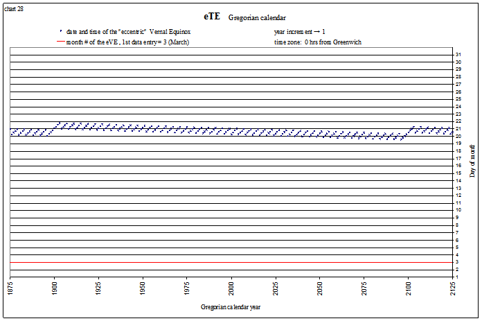
The following charts plot the dates and times of the 4 “tropical events” in the Gregorian calendar for ±30,000 yrs. They are calculated with “correct” mean orbital elements (using Laskar’s data beyond ±10,000 yrs). I have labeled these “eccentric” tropical events (eTE) to reflect that they are calculated from pure ellipse. Whereas I use “true” tropical event for a solstice or equinox calculated by the method of Bretagnon and Simon (1986), as these include the effects of our true orbit (perturbed by the Moon and planets).
|
Vernal Equinox
view larger→ eVE_Gregorian1.png |
Summer Solstice
view larger→ eSS_Gregorian1.png |
|
Autumnal Equinox
view larger→ eAE_Gregorian1.png |
Winter Solstice
view larger→ eWS_Gregorian1.png |
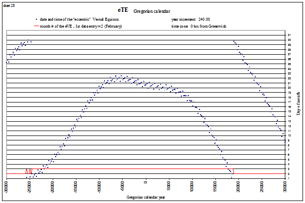
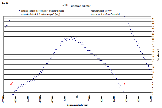
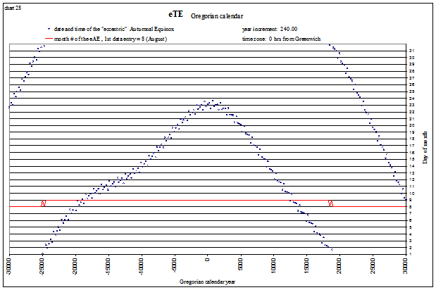
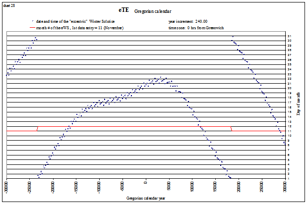
We see that the solstices and equinoxes start occurring in the “wrong” months after about 20,000 years (the red lines indicate the month#). This is mostly due to the slowing of Earth’s rotation rate, but why are the shapes of each curve different? Let’s look at a “fictitious” Gregorian calendar, one that assumes the day is not lengthening, for a longer time span and see if we can uncover the answer. The tropical events are shown below from −35,000 (35,001 BC) to 65,000 AD. The lines appear so smooth because one is plotted every 400 years, corresponding to our 400 year “leap year schedule”. The red line again indicates the month#. For example, the Vernal Equinox is shown below to be occurring in April (month# 4) at −30,000, and in February (month# 2) at +60,000:
|
Vernal Equinox
view larger→ fictVE.png |
Summer Solstice
view larger→ fictSS.png |
|
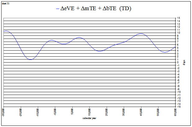
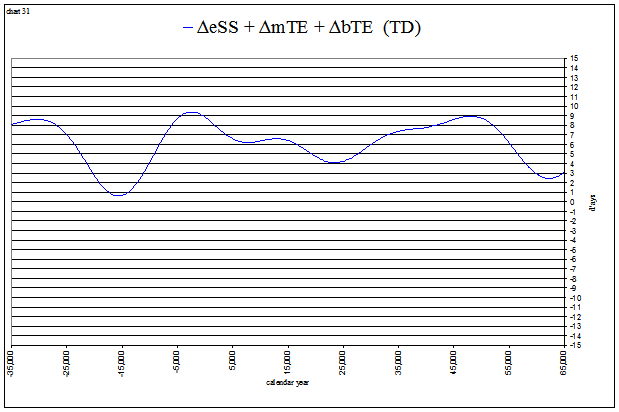
view larger→ delta_eVEplus.png |
view larger→ delta_eSSplus.png |
|
Autumnal Equinox
view larger→ fictAE.png |
Winter Solstice
view larger→ fictWS.png |
|
view larger→ delta_eAEplus.png |
view larger→ delta_eWSplus.png |
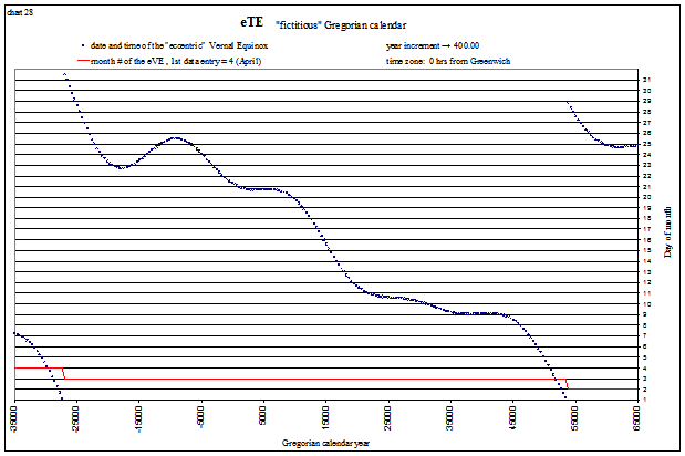
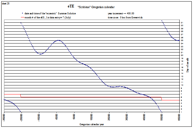
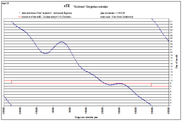
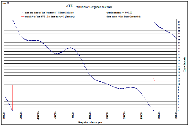
We can see from this short study that the solstices and equinoxes would remain in their “proper” months for about 50,000 years in the future, if Earth’s rotation rate did not slow down. The reason they still fall out of their respective months, even with this “fictitious” assumption that ΔT = 0, is of course that our calendar depicts the tropical year to be 365 97/400 (365.2425) days in length: slightly longer than an average tropical year of 365.242138.
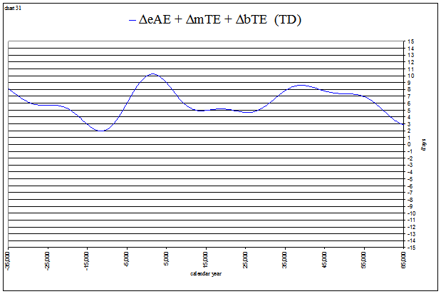
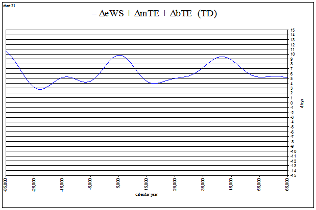
The general shapes of the curves are seen to correspond to the sum of 3 values. For the vernal equinox I’ve labeled them ΔeVE + ΔmTE + ΔbTE. (TD) indicates that these values are measured in days of dynamical time.
ΔeVE
measures the effects of the eccentricity and position of the perihelion upon
the vernal equinox. It is the difference, in time, between a vernal equinox
calculated in elliptical orbit, and one calculated in circular orbit. For an
unperturbed elliptical orbit it is the value ![]() , where C is the “equation of center” at a vernal equinox, and nt
is the “tropical” mean motion, measured as 360° per mean tropical year.
, where C is the “equation of center” at a vernal equinox, and nt
is the “tropical” mean motion, measured as 360° per mean tropical year.
ΔeSS
is ![]() where C is the equation of center at a summer solstice
where C is the equation of center at a summer solstice
ΔeAE
is ![]() where C is the equation of center at an autumnal
equinox
where C is the equation of center at an autumnal
equinox
ΔeWS
is ![]() where C is the equation of center at a winter solstice
where C is the equation of center at a winter solstice
ΔmTE measures the effects of the changing speed of the precession upon a solstice or equinox (tropical event, TE). It is the difference, in time, between a solstice or equinox calculated with the “true” precession in longitude, and one calculated with a long-term “average” precession rate. By the use of the solution La93(0,1) this long-term average rate is also constant, 50.4712 arcseconds per Julian year. This allows our simple study to remain quite simple (other of his solutions show this long-term average rate to be slowly decreasing).
ΔbTE measures the effects of the changing length of the sidereal year upon a solstice or equinox. It is the difference in time between a solstice or equinox calculated with a changing sidereal year, and one calculated with a constant long-term “average” sidereal year. Its effects are supposed to be very minor.
The values charted separately from −35,000 to +65,000 look like this:
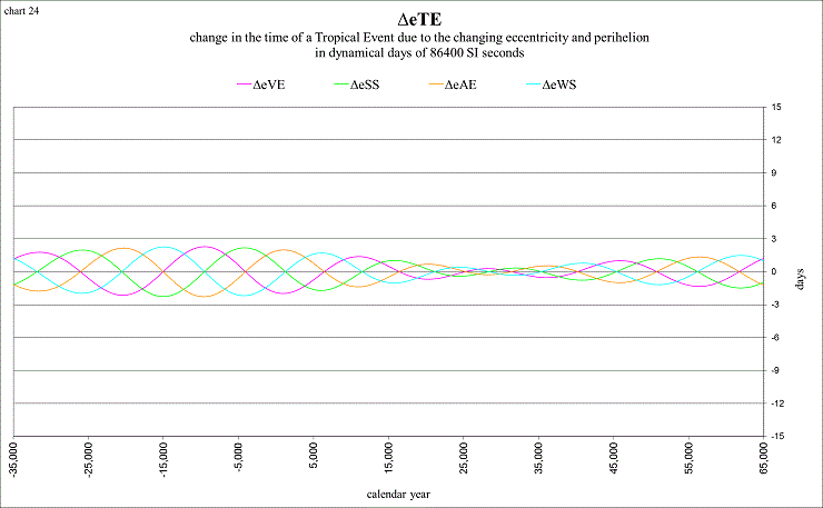
view larger→ delta_eTE1.png
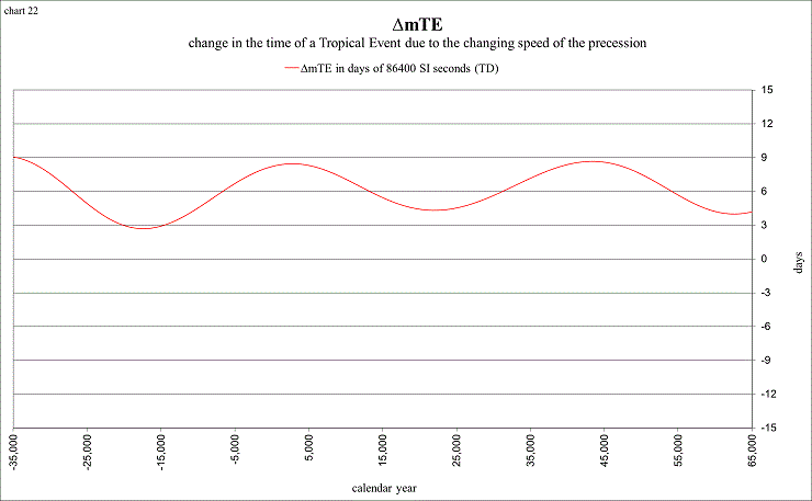
view larger→ delta_mTE1.png
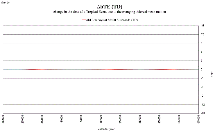
view larger→ delta_bTE1.png
These values charted together look like this:
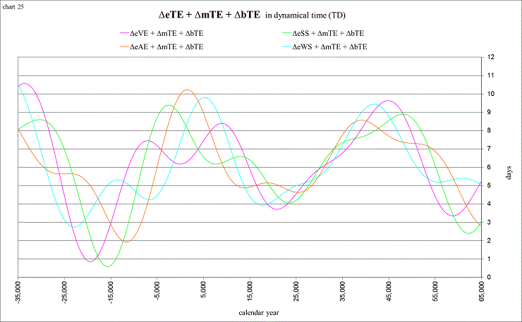
view larger→ delta_eTEplus.png
The reason ΔmTE is not currently centered around zero is that the precession in longitude shows general trends of “slightly faster” than average, and “slightly slower” than average, in regular cycles of ~4 million years. The next chart shows ΔmTE from −20M to +10M, using 1500 data points (all of the previous charts have used 250). Once again, it is the difference between the “true” precession in longitude, and an “average” precession in longitude described by 360° per 25678 Julian years (50".4712 per yr), converted to time and expressed as ‘days’ of dynamical time.
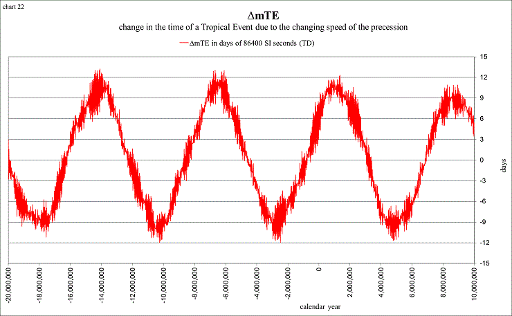
view larger→ delta_mTE2.png
What this chart is telling us is that about 3 million years ago the variations to the precession in longitude caused solstices and equinoxes to occur about 12 days sooner than average, and 1 million years in the future about 12 days later than average. The precession is currently causing them to occur about 8 days later than the long-term average.
To continue our study of solstices and equinoxes beyond 20,000 years, the spreadsheet creates a calendar, including the formulae you use to determine ΔT, so that it includes the effects of the slowing of Earth’s rotation rate. It’s basic “rules” are quite simple:
Place the “average” vernal equinox “mid-March”.
Place the “average” summer solstice “mid-June”.
Place the “average” autumnal equinox “mid-September”.
Place the “average” winter solstice “mid-December”.
By another “rule” it defines “mid-month” to currently be the 15th.
The next chart shows the values of ΔeTE + ΔmTE + ΔbTE converted to Universal time (or our estimation of UT) for ±100,000 years. It gives us a general idea of the changes in the day of the month that each solstice and equinox will occur in this calendar.
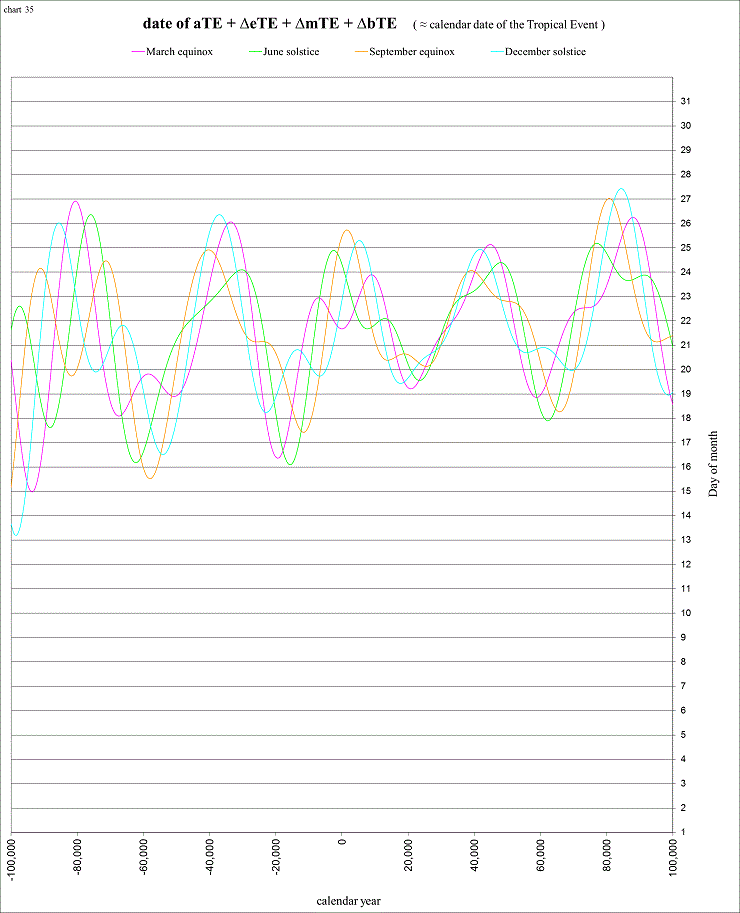
view larger→ calendar_dates.png
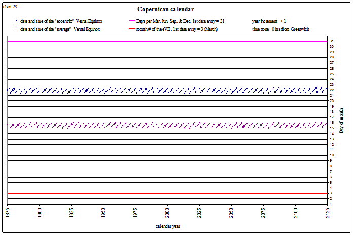
The next charts separately plot the date and time of each solstice and equinox in this calendar. I enjoy labeling this a “Copernican” calendar, as it assumes we are in “circular” orbit, making the “seasons” (the calendar quarters) equal in length. It also assumes that the length of the sidereal year is constant (unchanging), and that the rate of precession is constant, so that the length of the (average) tropical year is a constant length of dynamical time. I also rather like this label because he is often described as the progenitor of modern scientific advancement, as in the “Copernican Revolution”. One of the most profound modern discoveries (as far as a calendar is concerned) is that the Earth’s spin rate is slowing down, mostly due to tidal friction. To include this phenomenon in a calendar, and attribute it’s discovery to the Copernican Revolution, provides further enjoyment in labeling this a “Copernican calendar”. You, of course, can name it anything you like, change some of the “rules”, and create a calendar of your own. The “average” tropical events are also plotted, to make sure that they are currently occurring on the 15th of the month (in Greenwich).
This is the vernal equinox in the month of March:
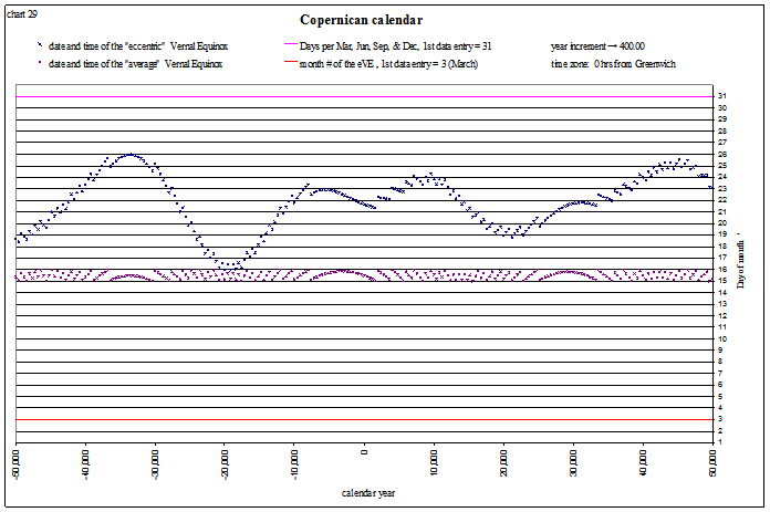
view larger→ eVE_Copernican1.png
This is the summer solstice in the month of June:
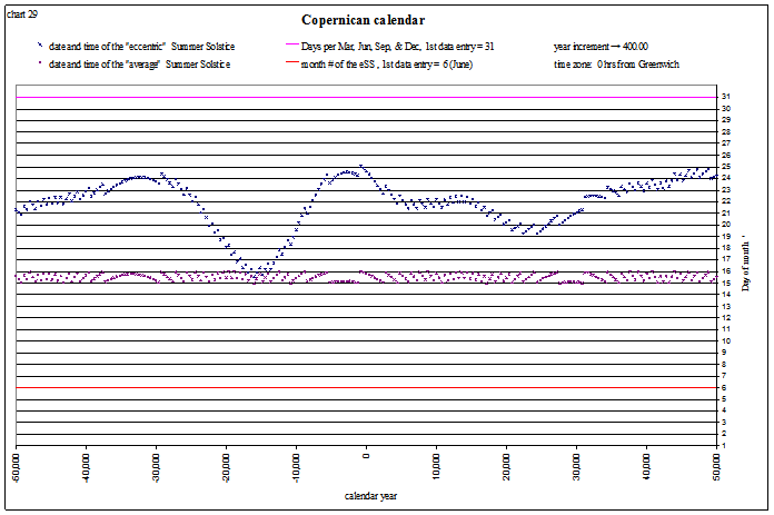
view larger→ eSS_Copernican1.png
This is the autumnal equinox in the month of September:
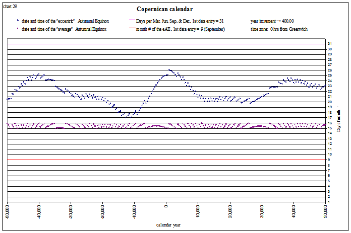
view larger→ eAE_Copernican1.png
And this is the winter solstice in the month of December:
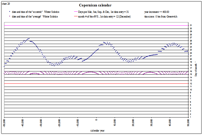
view larger→ eWS_Copernican1.png
It is interesting to inspect this calendar far into the past and future. The next chart shows the winter solstice 3 million years ago, when it can dip into the end of November by a few days:
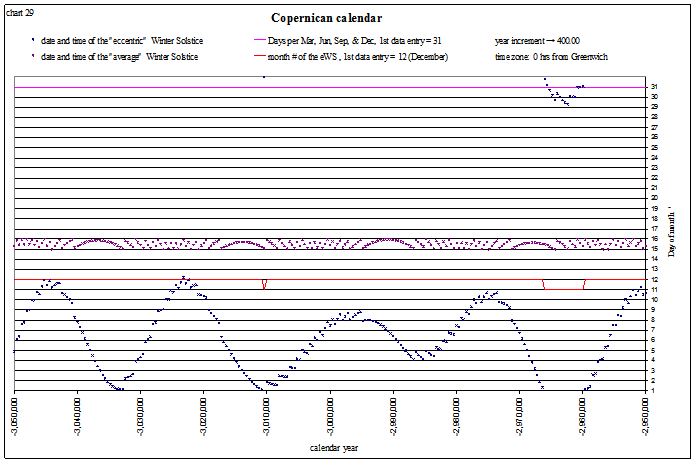
view larger→ eWS_Copernican2.png
And this charts the summer solstice 1 million years in the future, where it can occasionally occur during the beginning of July:
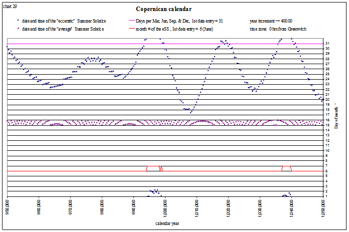
view larger→ eSS_Copernican2.png
This shows the long term “ups and downs” of the vernal equinox for the entire time span (−20M to +10M) of the orbital elements from Laskar’s 1993 data:
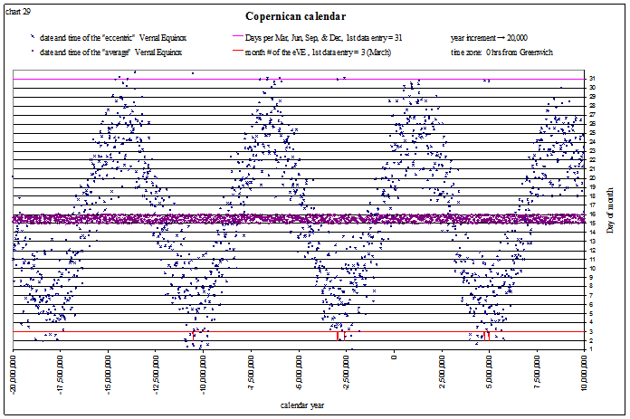
view larger→ eVE_Copernican2.png
Beyond −20M to +10M the solstices and equinoxes that the spreadsheet calculates are of course no longer valid (even though it continues to calculate them from the quasi-periodic approximation formulae), but it continues to count the days per year and divide the 12 months according to the “rules”. This particular scenario shows 482 days per year 686,000,000 years ago, and divides the 12 months into 38 days each, with mid-month defined as the 19th. 5 billion years in the future it shows 152 days per year, 13 days per month, with mid-month defined as the 6th.
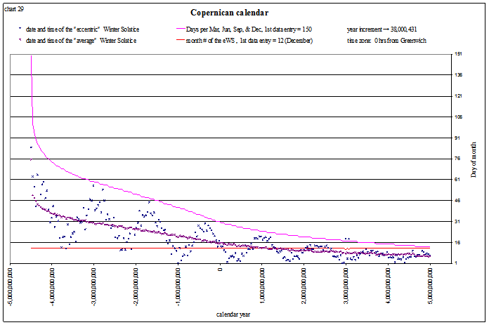
view larger→ eWS_Copernican3.png
Currently the vernal equinox in the calendar looks like this (at the longitude of Greenwich):
view larger→ eVE_Copernican3.png
The reason for the “regularity” is that this (currently) shows a “leap year” once every four years or once every five years, whereas the Gregorian calendar shows once every four years or once every eight years:
view larger→ eVE_Gregorian3.png
The different “scenarios” are best interpreted by the derivative of LOD, the rate that we are slowing, expressed as milliseconds per century. In the spreadsheet I am currently working on scenario 14a, as I believe it is one of the most realistic:
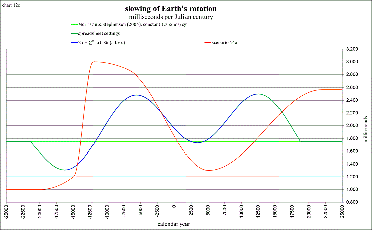
view larger→ ms_cy2.png
1.0 ms/cy is shown at −20,000 (20001 BC). It is supposed to represent the latter stage of the last ice-age. Our rate of slowing is supposed to be much less during glaciations (ice-ages), as the sea levels are lower, and most of the tidal friction occurs in the hydrosphere, which is mainly the oceans. From −20,000 to −3M the rate climbs slowly up to 1.4 ms/cy. This is intended to show an average rate of 1.2 ms/cy during the last 3 million years. It is a value suggested by Lourens et al (2001), from their study of core drillings in the Mediterranean Sea from 3 million years ago. This scenario then slowly increases to a more scientifically expected rate of 2.4 ms/cy at −3.5M.
At −20,000 (the minimum of 1.0 ms/cy in the chart above) the Earth’s shape is supposed to be in equilibrium. That is, she no longer needs to shift any more solid earth-mass from the polar regions into the equatorial region to compensate for the heavy ice loads at the poles and the lower sea level. The sharp increase to 3.0 ms/cy from −15,000 to −12,000 is supposed to represent the melting of the glaciers and the rising of the sea level. Imagine Earth to be like a spinning ice-skater. When the huge ice mass at the poles melts and sends the water mass towards the equator, this is like a spinning ice-skater slowly extending her arms, decreasing her measured moment of inertia and causing her to spin more slowly. The peak at 3.0 is supposed to represent the epoch in which the movement of water mass was at a maximum, and before “post-glacial rebound” was starting to have much effect.
The period between −12,000 and −8,000 is supposed to represent a combination of continued sea level rising and post-glacial rebound. From −8,000 to +22,000 (22,000 AD) the curve is supposed to represent our current era of post-glacial rebound (in which the ice-skater is drawing her arms inward causing her to spin faster). The Earth’s shape is shown to be back in equilibrium at +22,000, no longer needing to shift any more mass from the equator to the poles. It then continues on into the future at a scientifically expected rate of 2.4 ms/cy. The minimum of 1.3 is supposed to represent the epoch (about +5,000 in this scenario) in which the rate of movement of solid earth-mass (from post-glacial rebound) is at a maximum.
These rates and the epochs in which they are shown to occur are of course speculative. Due to a study of ΔT given by Morrison and Stephenson (2004), and the polynomials of Espenak and Meeus (from NASA) following that study, I am also working on a “sum of sines”, charted above as “2 r + ∑² -a b Sin(a t + c)”. It comes from the derivative the first two terms of the preliminary results of an LOD series I am working on, charted below as “2 r t + ∑¹⁴ b Cos(a t + c)”, a sum of cosines:
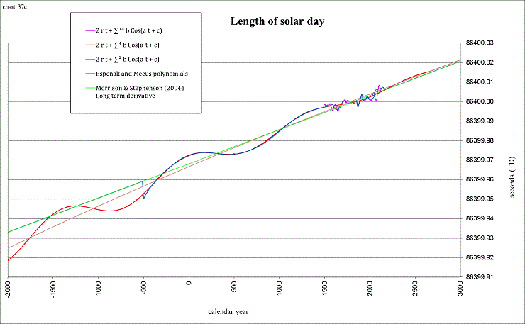
view larger→ LOD2.png
You can barely detect from this chart why I have chosen to use the Espenak and Meeus polynomials only until −404, even though they are given to −500. The next chart exemplifies this more clearly, as Morrison and Stephenson have given data (to be used with caution) until −2000:
view larger→ ms_cy1.png
Scenario 9b charted below uses the accuracy of the “sum of sines” for about ±20,000 years, then shows a constant rate of 1.75 ms/cy during the past 4.5 million years. My reasoning is this: if the average rate during the past 3 million years (from Lourens et al 2001) was 1.2 ms/cy and then the rate suddenly increased to as much as 2.6 ms/cy (from Laskar et al 2004), it would probably take at least another 1½ million years for the scenario’s rate of 1.75 to be showing the “correct” LOD at −4.5M. At −4.5M it simply steps up to the more scientifically expected rate of 2.5 ms/cy. Not being able to predict that the future will be much different than the past, it simply shows 1.75 ms/cy for 4.5 million years into the future, where it steps up to 2.5 ms/cy.
view larger→ ms_cy4.png
view larger→ ms_cy3.png
Scenario 9c is the same as 9b, but uses a simpler fraction to represent the length of the average tropical year (aty). 9b uses 365.2421378, while 9c uses 365 77/318 (365.24213836…). This is “allowed” for this spreadsheet, due to the fact that we don’t really know the true length of the long term average sidereal year (asy). This scenario uses 365.2563624… as the average sidereal year so that the average precession rate is still 50".4712/Julian year. The spreadsheet requires you to enter the fractional portions of asy and aty as proper fractions. 14a and 9b use 365 121069/500000 for the average tropical year so that the nicely rounded decimal representation of 365.2421378 is achieved. Using proper fractions is just something I enjoy, so you’ll have to put up with this little “quirk” of mine. Rather than “rounding” to seven decimal places, I have fun “rounding” to the simplest fraction that also rounds to the same seven decimals. A few scenarios use 365 1409/5819 for the average tropical year (= 365.24213782…).
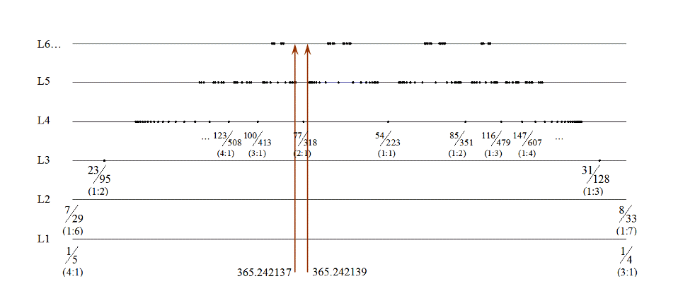
Since the true average length of the sidereal year remains unknown, I allow myself values between 365.256361 and 365.256363. At the average precession rate of 50".4712/Jyr (Julian year) this results in an average tropical year between 365.242137 and 365.242139. I then like to make a list of some of the simplest fractions that fall within this range. This is easiest to see from the “number line” that I use:
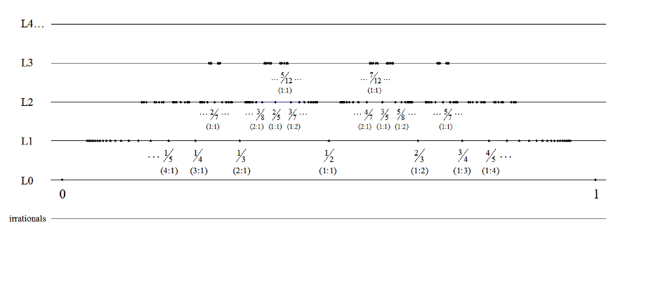
I split the
number line into specific separate number lines. L0 (level zero) is the
integers. L1 (level one) contains the simplest fractions. These are the same
“set” of fractions comprising the “outside shell” of the “farey tree”. It helps considerably to
understand the construction of the farey tree by means of a farey sum in order to easily grasp this number
line structure that I use. It is in fact a “flattened” farey tree, pushed flat
(and inverted). The values in parentheses below each fraction I refer to as
the ratio (x : y), where x
designates the number of “left-hand parents” and y designates the number
of “right-hand parents” used to construct the fraction by means of a farey
sum. For example, 4/7 is labeled (2:1). It belongs to
the “set” of level 2 fractions between 1/2 (the left-hand
parent of this set) and 2/3 (the right-hand parent). It
uses the left-hand parent twice and the right-hand parent once
(in a 2:1 ratio) to construct the fraction by means of a farey sum: ![]() . All of the “sets” of fractions on
L2 (level two) are the “subshells” of the farey tree that are once removed from
the outside shell. Each set of level 3 fractions is a subshell twice removed,
etc. Each “(1:1)” value is the mediant of each set, and is the apex of each
“shell” of the farey tree. I can “zoom in” to any portion of this structure to
view different portions of this “number line”. This view zooms in to a portion
around our upper and lower limits for the average tropical year:
. All of the “sets” of fractions on
L2 (level two) are the “subshells” of the farey tree that are once removed from
the outside shell. Each set of level 3 fractions is a subshell twice removed,
etc. Each “(1:1)” value is the mediant of each set, and is the apex of each
“shell” of the farey tree. I can “zoom in” to any portion of this structure to
view different portions of this “number line”. This view zooms in to a portion
around our upper and lower limits for the average tropical year:
This view zooms in a little closer:
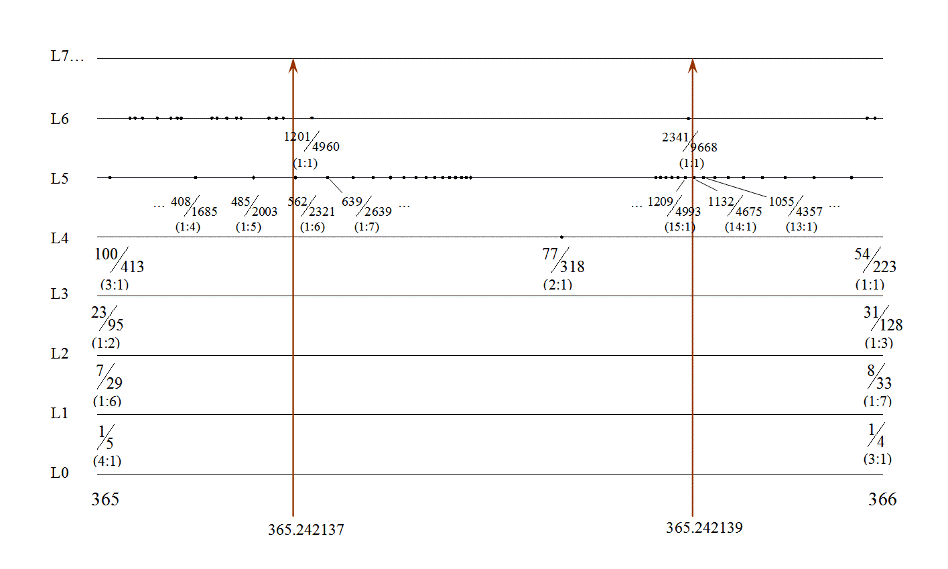
This begins a list of some of the simplest fractions within our range. When one is familiar with the construction of the farey tree it is quite simple to determine all of the fractions corresponding to the points not labeled above. The top portion of sheet f! in the spreadsheet is a tool I use to navigate this number line, and is separate from the main portion of the spreadsheet. It uses the following algorithm to find the placement of any rational number within this structure:
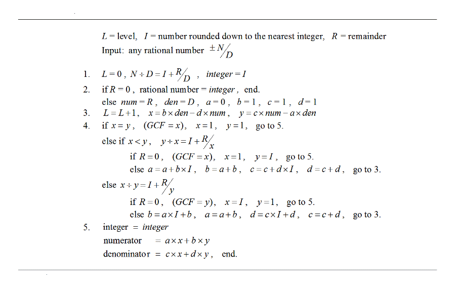
![]() (from line 5.) is a fraction’s
“definition”, and will always be in it’s proper “reduced” form, the same as all of the fractions from the farey tree. (GCF) indicates the point in the algorithm where the
greatest common factor can be determined, even
though it is not used to display the fraction in its proper reduced form.
(from line 5.) is a fraction’s
“definition”, and will always be in it’s proper “reduced” form, the same as all of the fractions from the farey tree. (GCF) indicates the point in the algorithm where the
greatest common factor can be determined, even
though it is not used to display the fraction in its proper reduced form. ![]() is used. It is not necessary to
understand this in order to use the spreadsheet. The bottom portion of sheet
f! does use this algorithm and is part
of the main spreadsheet. I could have more
easily used a “continued
fraction” algorithm
for the bottom portion, but I just recently learned about continued fractions,
so for now I’ve left it as it is. A continued fraction finds the closest
fraction (to the number in question) on each successive level of this
structure, whereas this “construction algorithm” finds the two that are
closest, a/c & b/d . It is
of course between the two, and in fact constructed (by means of a farey sum) of
the two it is between, on each level. The Excel file ConstructionAlgorithm(xn).xls
is the same as the top portion of sheet f!, but with the precision of Xnumbers
(a required Add-In available from Foxes Team that can calculate to a precision of
up to 250 significant digits), for anyone interested in delving into deeper
levels of this structure.
is used. It is not necessary to
understand this in order to use the spreadsheet. The bottom portion of sheet
f! does use this algorithm and is part
of the main spreadsheet. I could have more
easily used a “continued
fraction” algorithm
for the bottom portion, but I just recently learned about continued fractions,
so for now I’ve left it as it is. A continued fraction finds the closest
fraction (to the number in question) on each successive level of this
structure, whereas this “construction algorithm” finds the two that are
closest, a/c & b/d . It is
of course between the two, and in fact constructed (by means of a farey sum) of
the two it is between, on each level. The Excel file ConstructionAlgorithm(xn).xls
is the same as the top portion of sheet f!, but with the precision of Xnumbers
(a required Add-In available from Foxes Team that can calculate to a precision of
up to 250 significant digits), for anyone interested in delving into deeper
levels of this structure.
I am sure there are other “oddities” in this spreadsheet, as I am not an expert user of Excel (e.g. I just discovered the “formula auditing toolbar”: how did I ever get along without it?!). I am also not by any means an expert in astronomy, so that some things are undoubtedly “shortcuts”, while many more things are probably on the order of “taking the long way around”:
For example, when I first started this project I posed the question to myself: “if I were an ancient astronomer, how would I build a calendar?” First I would ask the wisest and most knowledgeable high priests and astronomers all that they knew about the length of the year and the lengths of the seasons. I would undoubtedly have found out that while the shortest season was currently the fall season, our ancient ancestors might have measured the summer to be shortest (we had extensive records), and in the future winter will probably be shortest (as it is today), and on and on. Desiring this calendar to work for many millennia, it would become obvious that “equal quarters” would be the best solution, so that the solstices and equinoxes (the divisions of the seasons) would differ from the calendar’s equal “divisions of the quarters” by only a few days, sometimes sooner and sometimes later, depending upon the changing lengths of the seasons. But how would we start this calendar “correctly”? Simply set the vernal equinox on the same date as its representative “quarter division”? It seems that it should fall a day or so ahead or behind of its calendar representation, just the same as the other tropical events. Today we can use the equation of center and convert it to time, but the ancient astronomer would not have known Kepler’s equation, and might not have deduced that we were in orbit, let alone elliptical orbit! But simply from a “list” of the different lengths of the seasons he could easily have deduced the following relationships:
|
||||
|
|
||||
|
|
||||
|
|
||||
|
|
||||
|
|
And he would
have been absolutely correct! You can check that these relationships are exact
by making a “list” of the lengths of the seasons, at any given instant (epoch), by use of Kepler’s equation. If
you use the “true” lengths of the seasons (from our “perturbed” orbit), you
will find that the ancient astronomer’s method gives somewhat of an
approximation to the angular difference (true “perturbed” planet) − (mean
planet), while the equation of center gives the angular difference (true
“unperturbed” planet) − (mean planet). His determination of the equation
of center at a solstice or equinox is ![]() × 360°. And of course I use
this method in the spreadsheet, simply because it is fun! I also understand it better: calculating the lengths of the seasons by use of Kepler’s equation I simply look at as “magic”, as I have absolutely no idea how he came up with his famous
formula. I also look at Laskar’s approximation formulae as “magic”. From my
meager point of view (in regards to his formulae’s use of complex numbers):
× 360°. And of course I use
this method in the spreadsheet, simply because it is fun! I also understand it better: calculating the lengths of the seasons by use of Kepler’s equation I simply look at as “magic”, as I have absolutely no idea how he came up with his famous
formula. I also look at Laskar’s approximation formulae as “magic”. From my
meager point of view (in regards to his formulae’s use of complex numbers):
“This high priest in France
makes all numbers dance…
to the square root of negative one!”
There is only one more (extreme) “oddity” that requires discussion, and this involves the unknown changes to our semi-major axis (and therefore the unknown changes to the length of the sidereal year). From (what portions I can understand of) Laskar’s publications, his model of the solar system is a “second order general theory”, and that it would require a third order theory to accurately detect the changes to the semi-axes of the planets. And that it would be right next to impossible to even think about the integration of the equations of motion to the third order with respect to the masses of the planets for millions and millions of years! In order to derive his polynomial description for ±10,000 yrs (Laskar, 1986), (from what I can understand) the third order from existing classical theory was considered. My first idea to extend the known changes beyond ±10,000 came from the title of the article “fitting a line to a sine” by J Laskar and J-L Simon, 1988. My intention was to show (by a simple sine wave) the semi-axis returning to an “average” at about ±35,000 and then simply continuing with the constant, unchanging average beyond that range. This, however, produced an ugly “blip” in some of the charts: whereas the frequency of the integral is the same, it is exactly out of phase. To continue with this same sine function for millions of years removed the “blip”, but was endlessly boring, showing the same frequency and amplitude year after year after year. Simply to relieve my boredom, I decided to use the frequencies from the inclination variables from the quasi-periodic approximation formula from Laskar et al (2004), as they also show frequencies of about 70,000 yrs. It is important to note that this is not a scientific method, it is more on the order of “pick a formula, any formula” and force it to fit. The amplitudes have been adjusted in an extremely unscientific manner, simply to show some slight variation, and to “agree” with any reasonable choice for a “long term average sidereal year”. Once again, the description of the sidereal year in this spreadsheet is to be considered fictitious beyond ±10,000 yrs. It is used merely for interest, to depict a “possible” history of amplitudes, and to continue calculating in a “correct” manner, which would include our changing semi-major axis. If you would rather not use this fictitious rendition, it is very easy to direct the spreadsheet to calculate with the average sidereal year, and ∆bTE will simply always equal zero. The additional “error” in calculating a solstice or equinox, during ±10,000 yrs from J2000, without using the “correct” length of the sidereal year (from Laskar 1986) is only about 1½ hours of time.
view larger→ semi-axis.png
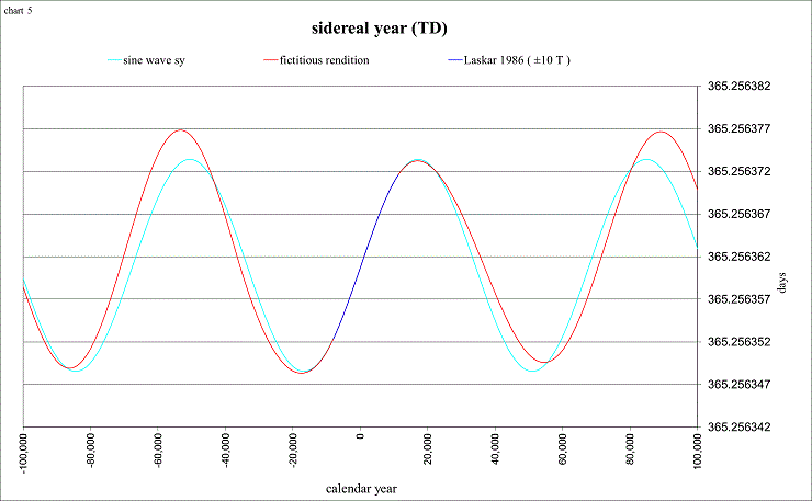
view larger→ sid_yr.png
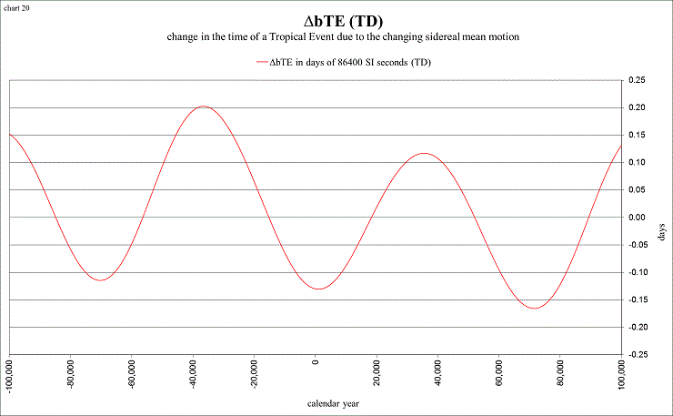
view larger→ delta_bTE2.png
∆bTE involves the integral of the (changing) sidereal year. At ~1000 AD the sidereal year is shown to be at the average, while ∆bTE is at a minimum, due to the previous 35,000 years, during which time the sidereal year was below average.
References
Bretagnon, Pierre, and Jean-Louis Simon, 1986, Planetary Programs and Tables from −4000 to +2800, Willmann-Bell, ISBN 0‑943396‑08‑5
Canup, R., 2004, Origin of the Terrestrial Planets and the Earth-Moon System, Physics Today 57, (April 2004) 56‑61 (pdf)
Deubner, F.-L. : 1990, Discussion on Late Precambrian tidal rhythmites in South Australia and the history of the Earth’s rotation, J. Geol. Soc. London, v. 147, no. 6, 1083‑1084
Dickey, J.O., P.L. Bender, J.E. Faller, X.X. Newhall, R.L., Ricklefs, J.G. Ries, P.J. Shelus, C. Veillet, A.L. Whipple, J.R. Wiant, J.G. Williams, C.F. Yoder, 1994, Lunar laser ranging: A continuing legacy of the Apollo program, Science, 265, 482–490
Laskar, J., 1985, Accurate methods in general planetary theory. Astron. Astrophys. 144, 133–146
Laskar, J., 1986, Secular terms of classical planetary theories using the results of general theory. Astron. Astrophys. 157, 59–70
Laskar, J., 1988 Secular evolution of the Solar System over 10 million years. Astron. Astrophys. 198, 341–362
Laskar, J. and J-L. Simon, 1988, Fitting a line to a sine, Celest. Mech., 43, 37–45
Laskar, J., 1990, The chaotic motion of the Solar System: a numerical estimate of the size of the chaotic zones. Icarus 88, 266–291
Laskar, J., Joutel, F., Boudin, F., 1993, Orbital, precessional, and insolation quantities for the Earth from −20 Myr to +10 Myr. Astron Astrophys. 270, 522–533
Laskar, J., Robutel, P., Joutel, F., Gastineau, M., Correia, A., Levrard, B., 2004, A long term numerical solution for the insolation quantities of the Earth, Astron. Astrophys., 428, 261–285 December(II) 2004
Lourens, Lucas J., Rolf Wehausen, Hans J. Brumsack, 2001, Geological constraints on tidal dissipation and dynamical ellipticity of the Earth over the past three million years. Nature 409, 1029-1033
Meeus, Jean, 1998, Astronomical Algorithms 2nd ed., Willmann-Bell, ISBN 0-943396-61-1
McCarthy, Dennis D., Precision time and the rotation of the Earth, Transits of Venus: New Views of the Solar System and Galaxy Proceedings IAU Colloquium No. 196, 2004, D.W. Kurtz, ed.
Morrison, L.V., Stephenson, F.R., 2004, Historical values of the Earth's clock error ΔT and the calculation of eclipses, Journal for the History of Astronomy 35, 327–336
Munk,Walter, 2002, Twentieth century sea level: An enigma, PNAS, May 14, 2002, vol. 99 no. 10, 6550–6555
Nelson, R. A. et al, 2001, The leap second: its history and possible future, Metrologia, 38, 509–529 (pdf)
Néron de Surgy, O., Laskar, J., 1997, On the long term evolution of the spin of the Earth. Astron. Astrophys., 318, 975–989
Quinn, T. R., S. Tremaine, and M. Duncan, 1991: A three million year integration of the Earth’s orbit. Astron. J., 101, 2287−2305
Simon, J.-L., Bretagnon, P., Chapront, J., Chapront-Touze, M., Francou, G., Laskar, J. : 1994, Numerical expressions for precession formulae and mean elements for the Moon and the planets. Astron. Astrophys., 282, 663-683
Sonett, C. P., E. P. Kvale, A. Zakharian, M. A. Chan, and T. M. Demko, 1996, Late Proterozoic and Palaeozoic tides, retreat of the Moon, and rotation of the Earth, Science, 273, 100–104
Stephenson, F. R., 1997, Historical Eclipses and Earths Rotation, Cambridge University Press, 64
Stephenson, F.R., 04/2003, Harold Jeffreys Lecture 2002: Historical eclipses and Earth’s rotation. Astronomy & Geophysics, 44 (2) 2.22–2.27
Walker, J.C.G. & Zahnle, K.J., 1986, Lunar nodal tide and distance to the Moon during the Precambrian. Nature, 320, 600–602
Williams, G.E., 1989, Tidal rhythmites: geochronometers for the ancient Earth-Moon system. Episodes, v.12, no. 3, 162–171
Williams, G.E., 2000, Geological constraints on the Precambrian history of Earth’s rotation and the Moon’s orbit: Reviews of Geophysics, 38, 37–59 (pdf)
Notice: due to a Windows security measure all of the zipped files that you download might be “blocked”. Before unzipping right-click the .zip, choose “Properties”, then in the “General” tab click “Unblock”, “Apply”, and “OK”. Otherwise you might need to perform these steps on each individual file (especially .chm helpfiles).
If you are interested in using the Excel Add-In for the interpolation of Laskar’s La93(0,1) data from −20M to +10M, you can read a description of the functions in OrbitalElements1.7.pdf, and download OE.xlam1.7 for Excel 2007/2010, or OE.xla1.7 for 97/2000/XP/2003. This newer version 1.7 has a bug fix for Excel 97 & 2000. If you would like to use the spreadsheet that created the charts on this webpage, you can read the “short” instructions to start, and download ECT1.6.xlsm for Excel 2007/2010, or ECT1.6.xls for Excel 97/2000/XP/2003. If you are interested in the method being used to calculate the approximate times of solstices and equinoxes, download TEequation.pdf. This updated pdf also contains a new ΔT section with readjusted “double precision” formulae for the entire time span −4.5G to +5G. There are two additional Add-Ins required to use this workbook. The 1st is “Analysis Toolpak” (on your Office CD if it isn’t already installed), in order to read the function “SERIESSUM( )”. The 2nd is “Xnumbers v.6.0”, a remarkable math tool for Excel.
All of these Add-Ins are being distributed as open source, fully accessible to modify and redistribute as you desire, as long as you give credit to the original authors, Leonardo Volpi from Foxes Team for the Xnumbers Add-Ins, and John Beyers for the Orbital Elements Add-Ins.
For any other questions or comments, or (if you aren’t too comfortable with Excel and/or all of these Add-Ins) to request custom charts (in Word), and/or data to create them (in Excel) for specific time spans and parameters: email to steve@thetropicalevents.com. Please be very patient to receive a reply, as I am usually at home, a “little cabin in the woods”, with my dog Tuxedo, far from the city lights (and an internet connection).
Thanks for your interest,
![]()
|
|
|


P.S. to help bring an “ancient astronomer” (or “old carpenter who uses fractions”) up to date in the modern world, don’t hesitate to donate to the solar system (electric) and satellite (internet connection) fund!
For a printable version of this webpage use TropicalEvents.pdf
Other interesting websites:
http://www.imcce.fr/Equipes/ASD/person/Laskar/Laskar.html
Laskar’s website
ftp://ftp.imcce.fr/pub/ephem/sun/la93
has the ASCII files with the data (used in this spreadsheet) from La93(0,1), given every thousand Julian years, −20M to +10M from J2000. They are in a compressed format, *.ASC.Z
http://adc.gsfc.nasa.gov/adc-cgi/cat.pl?/catalogs/6/6063/
has the same ASCII files in a different compressed format, *.ASC.dat.gz
ftp://cdsarc.u-strasbg.fr/pub/cats/VI/63
has the same, larger uncompressed ASCII files, *.ASC, easily imported to EXCEL
http://www.bowdoin.edu/~rdelevie/excellaneous/
Advanced Excel for scientists and engineers by Robert de Levie
http://www.astrosociety.org/education.html
Astronomical Society of the Pacific
http://www.astrosociety.org/education/publications/tnl/45/globe1.html
great educational site for astronomy
http://www.intute.ac.uk/sciences/astronomy/
another good educational site
http://www.astronomynotes.com/
and another
http://www.astrophysicsspectator.com/
The Astrophysics Spectator
Great learning site
http://www.amsat.org/amsat/keps/kepmodel.html
Keplerian Elements Tutorial
http://www.daviddarling.info/encyclopedia/C/celestial_mechanics_entries.html
awesome encyclopedia of celestial mechanics
http://individual.utoronto.ca/kalendis/seasons.htm
great charts of the seasons and years! Also a good variety of astronomical calendars
http://www.iol.ie/~geniet/eng/season.htm
lengths of astronomical seasons
http://webexhibits.org/calendars/
good info on astronomy and calendars
http://www.maa.mhn.de/Scholar/calendar.html
Astronomical Calendars: good basic info
http://www.ecben.net/calendar.shtml
huge list of different calendars
http://www.calendarhome.com/clink/general.html
good general calendar information
http://www.calendarhome.com/clink/reform.html
calendar reform
http://personal.ecu.edu/mccartyr/calendar-reform.html
calendar reform
http://www.astro.uiuc.edu/projects/data/
fun demos and animations
http://seds.lpl.arizona.edu/nineplanets/nineplanets/nineplanets.html
A Multimedia Tour of the Solar System
interesting and widely referenced astronomy site
Steve Beyers
145 Electric Ave
Seal Beach, CA 90740
USA
last updated December 5, 2010